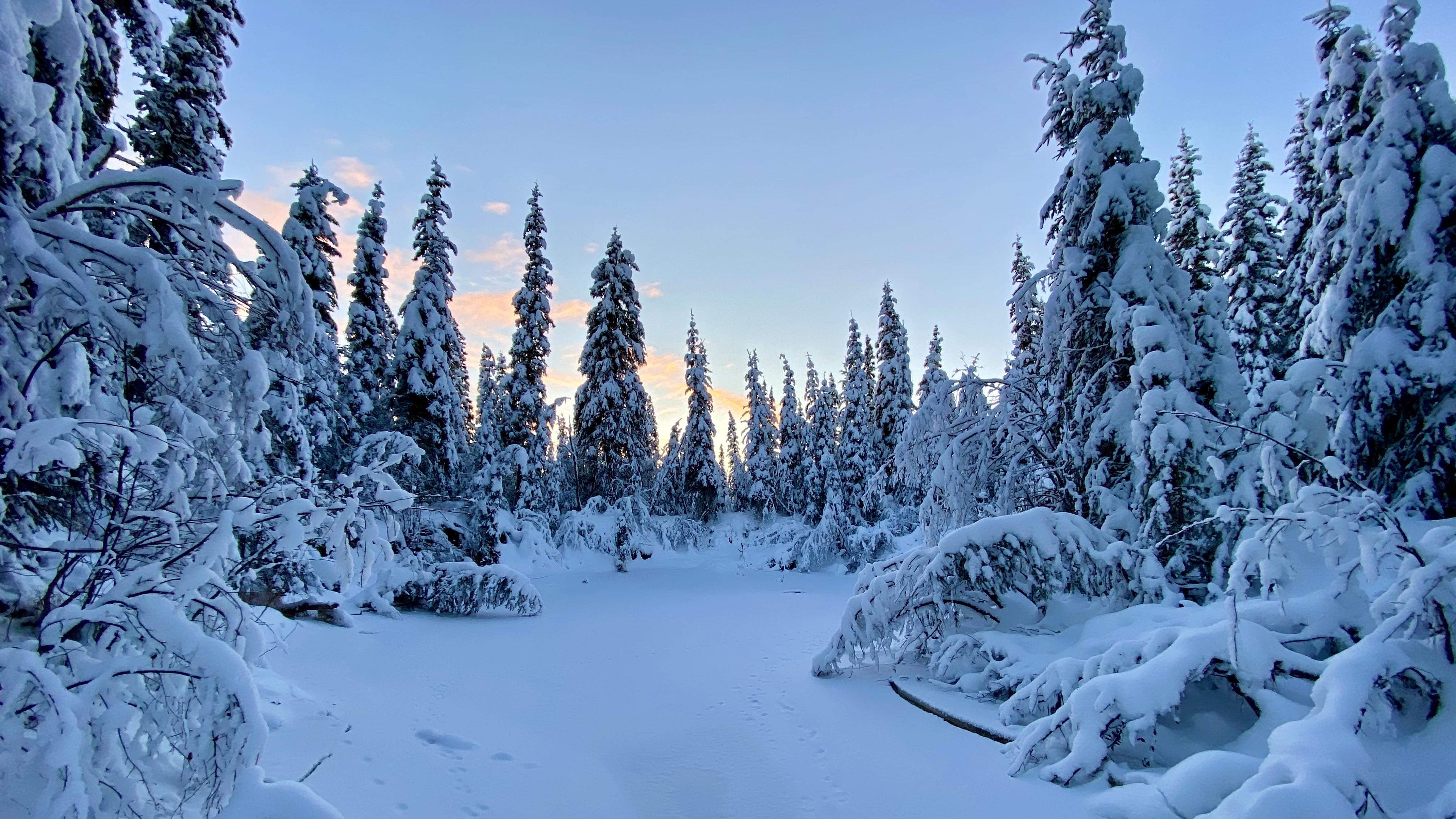
Yesterday I went for my first run on Goldstream Creek this winter and noted a very smooth descending line on the elevation diagram from my Garmin watch while I was on the creek. There was a significant overflow event on November 29th, and with the cold temperatures since then, the water on the surface froze solid.
Here’s the plot of creek height and temperature for the last seven days. You can see the overflow event on November 29th, and a sudden drop starting yesterday afternoon.
Usually when there are overflow events like this they are fairly restricted, overflowing in one place for a thousand feet or so, freezing, then overflowing somewhere else. But this event was large enough that I was running on clean ice for almost the entire time I was down on the Creek. In winter, I run with Black Diamond Distance Spikes, and barely slip at all, even on smooth ice.
Here’s the map of my run.
And the elevation diagram. You can clearly see where I dropped down onto the Creek at the end of Miller Hill/Miller Hill Extension at a quarter mile, and then came back up at the Murkowski cabin near mile 2¼. The orange line shows a fitted line to the elevation points while I was down on the Creek.
When I dropped down on the Creek at the end of Miller Hill and Miller Hill Extension, the elevation of the Creek was 562 feet, and 1.9 miles downstream it was down twelve feet to 550. The slope of the line is -5.876, indicating that the Creek drops almost six feet per mile along the course I ran.
Something happened to the ice overnight, at least at our house, so it’ll be interesting to check it out on my run today. The overflow on November 29th was around 4 inches deep, and last night it dropped almost the same amount. Since the surface is frozen, there must have been a layer of air under the ice that was filled with water earlier in the week, but after the water overflowed (and froze), that layer emptied and the ice on the surface dropped back down.
Martin
We let Martin go this afternoon after a long struggle with an inflammatory bowel disease. He came to us with his sister Piper nine years ago and was a strong and fast sprint dog known as one of the louder dogs at the track. He retired from racing in 2019 and enjoyed his remaining days sleeping on the futon and couch, often with a cat or his sister.
Martin was born in Salcha, Alaska on May 10, 2009 and won several races with Piper. He was known as the "ten thousand dollar dog" because he got torsion when he was young and the surgery to save his life was very expensive (along with later surgery and vet appointments investigating his digestive issues). He had the most beautiful, fluid trot running up and down the dog yard, but when he'd get into a race he was obsessive about being as far to the left as he possibly could, sometimes running halfway off the trail.
He liked beer, digging large holes in the dog yard so he could eat dirt, and would make playful growling noises when you scratched just the right spots on his hips. He got along with the cats, snuggling with them on the couch, and despite being fairly high on the hierarchy of our dogs, he was never aggressive about food or toys. He was the sweetest, softest dog we've had and was not only my favorite, but was the favorite of our UPS driver who pointed him out to Andrea one day and said, "That one is my favorite!"
Rest in peace buddy.
Martin at the Tok Race of Champions
Jenson and Martin on the couch
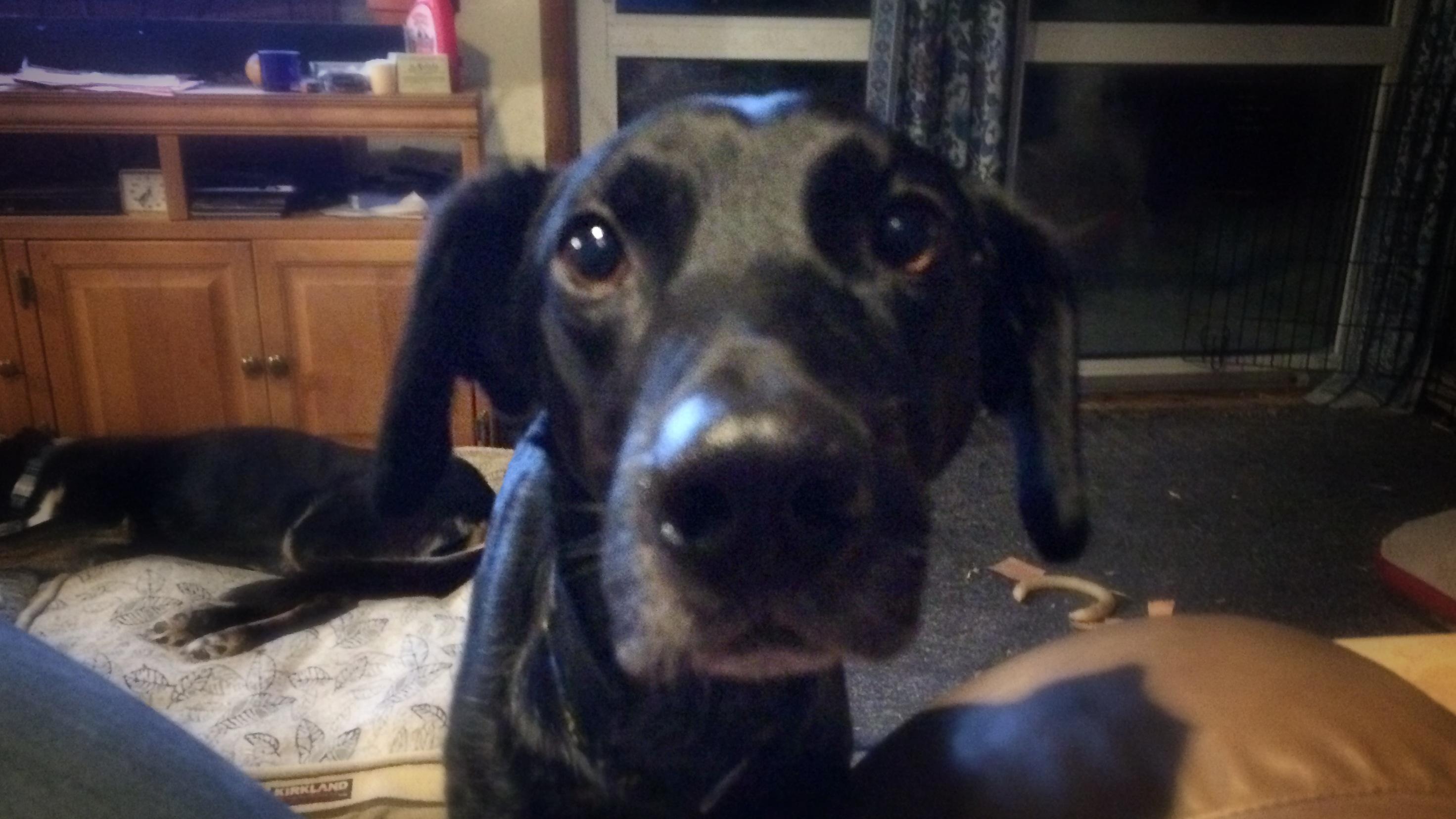
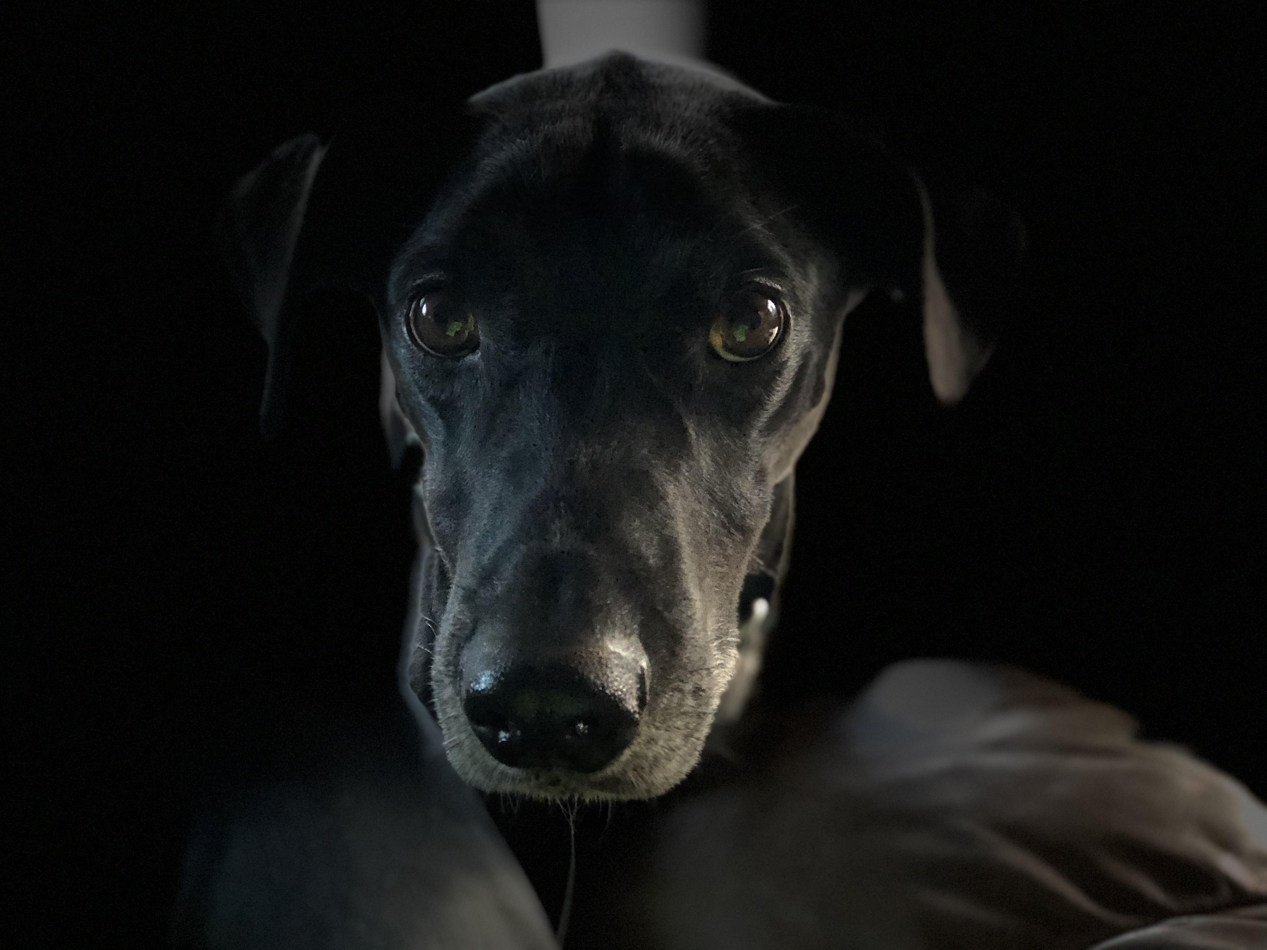
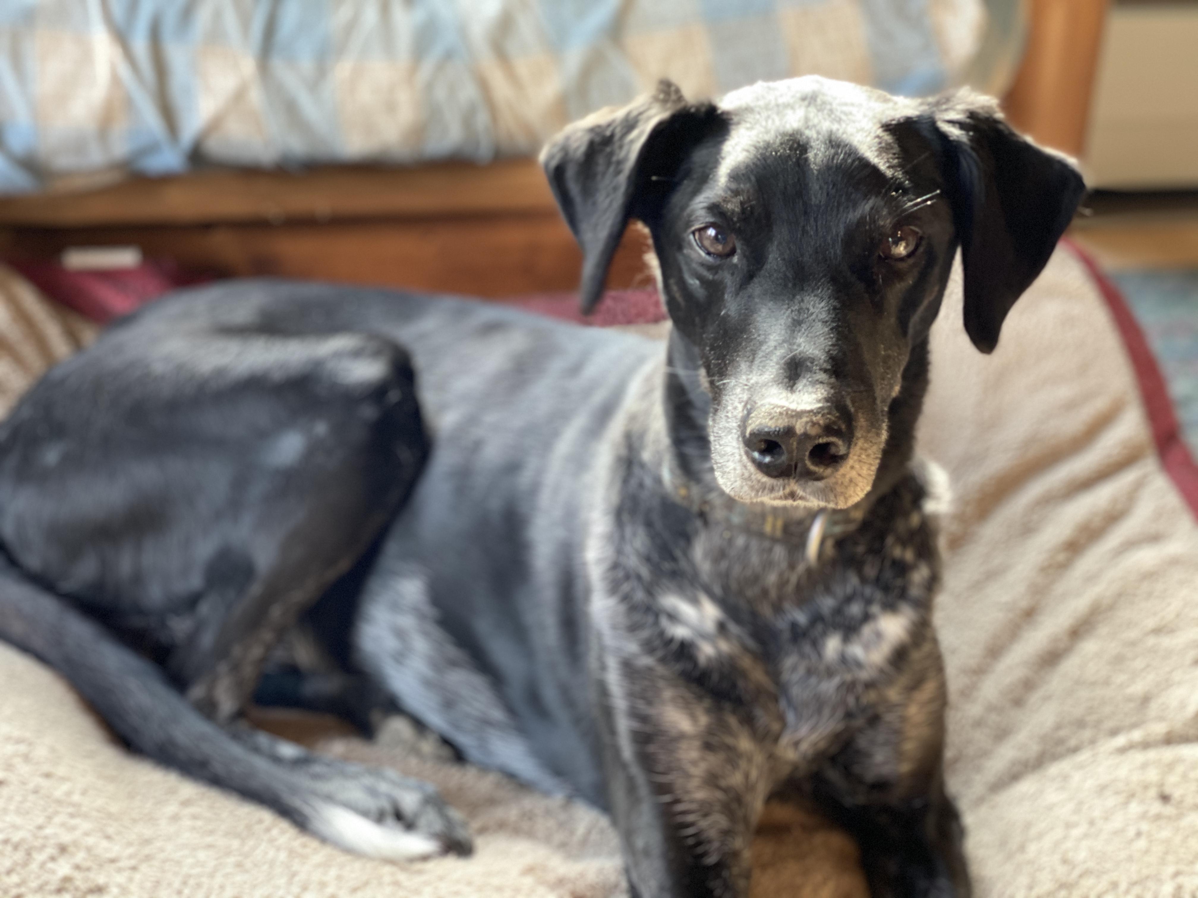
Martin's curious face
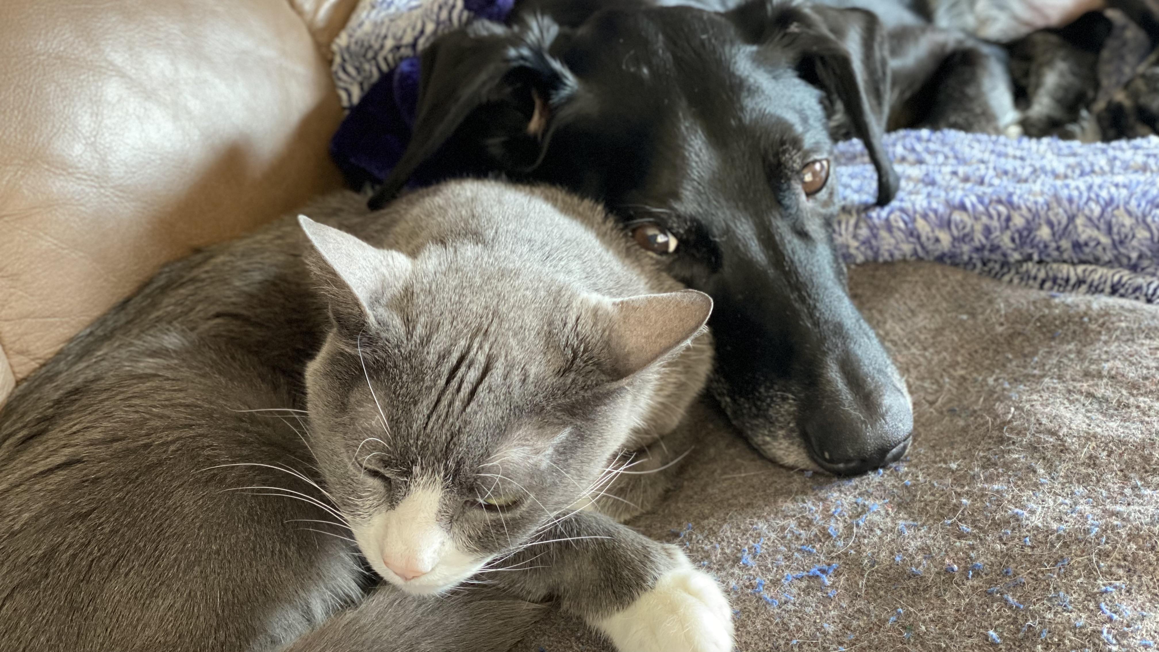
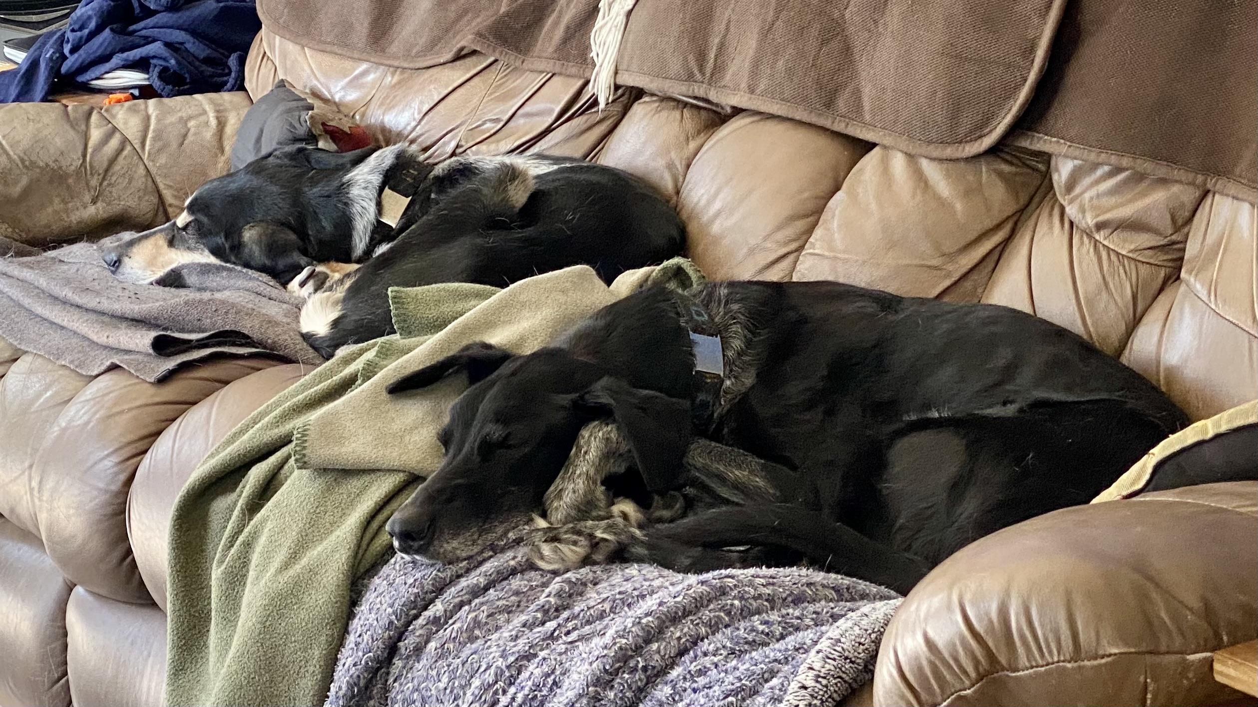
Tallys and Martin sharing the couch
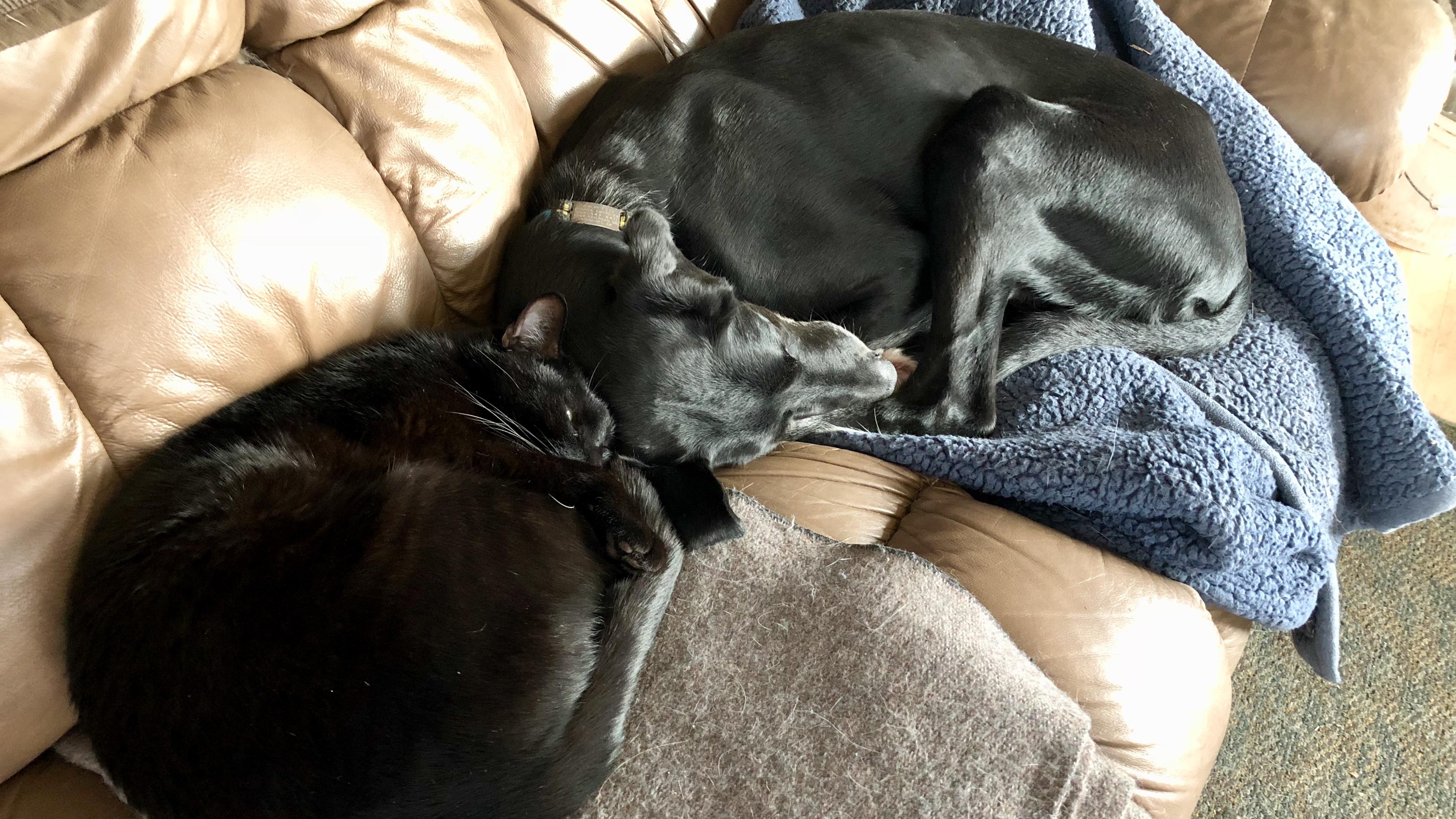
Martin and his sister on the couch
Martin
Problem
This morning I woke up about 20 minutes late because my iPhone 11 crashed overnight while sitting on my charger. That's the first time I've every had an iPhone crash. After using the “volume up”, “volume down”, “hold power button” trick, the phone came back up. I quickly installed the latest Apple update 16.3.1, just in case I’d stumbled into a bug that has been fixed.
Before I got it running again I thought about having to buy a new phone and what I might lose because I wouldn’t be able to copy the data from the old phone to the new one. I’m relying on iCloud Backup for most of the important things (photos, mostly), and all of my passwords and pretty much all of the data I care about is in git or in databases on my server, so losing the phone wouldn’t affect any of that.
But I have two factor authentication with Google Authenticator set up for several important sites, and I would have no way to get this “factor” back if the phone was truly dead. When I upgraded to this phone several years ago I sent back my previous phone to Apple and didn’t realize Google Authenticator “data” only exists on that one device. Oops. Sort of the point, if I’d thought about it.
Solution
Google Authenticator has a mechanism for transferring its data to a new device. You click the three dots in the upper right corner, choose “Export accounts”, then scan the QR code that shows on the screen with the new device.
Instead of scanning it, I took a screenshot, edited the photo, downloaded it to my computer, converted it to a PNG, encrypted it to plain text, added it to my password store, then deleted the image. This is sort of overkill since I'm encrypting the image data, then my password manager is encrypting it again. Alternatives include converting the image to text using uuencoding, or Eric Raymond's PNG to text converter, but doing it this way only requires tools I'm always going to have (GNU Privacy Guard and pass)
Here’s what the process looks like.
# Convert to a PNG (probably not necessary, but it's *data* so...)
$ convert -quality 100% IMG_0112.jpeg google_auth_qr_2023-02-15.png
# Encrypt
$ gpg --encrypt --armor google_auth_qr_2023-02-15.png
$ rm google_auth_qr_2023-02-15.png
# Add to password store (-m means multi-line)
$ cat google_auth_qr_2023-02-15.png.asc | \
    pass insert -m Internet/google-authenticator/qr_2023-02-15.png
$ rm google_auth_qr_2023-02-15.png.asc
If I ever need to recover it in the future, I do the reverse, which looks like the following.
$ pass Internet/google-authenticator/qr_2023-02-15.png > /tmp/foo.png.asc
$ gpg --decrypt /tmp/foo.png.asc > /tmp/foo.png
References
Caslon in a box
Caslon died today after a long fight with multiple myeloma. We got him as part of a foster litter with his brothers Jenson and Tallys. We’d chosen his brothers from the litter as kittens, but when we saw Caslon alone in his crate at the shelter after the rest of his brothers and sisters had been adopted, we couldn’t leave him there by himself. He was never quite as snuggly as his brother Tallys, who died in 2019, but he was the biggest and most playful of our cats. He always ate his food up on the cat tree and would jump up there with such force that he’d almost tip over the whole thing.
Once Tallys was gone he took over Tallys’s spot in front of the wood stove, and would request to be picked up every morning while I made coffee. He loved being under the covers on the guest bed, on the couch with Andrea, and sometimes in the middle of the night purring and kneading under the covers with Andrea. And while the dogs ate their dinner, he’d bolt over to one of the dog beds, flop and wriggle, and I’d give him super rubdowns. He was also the cat who always tested the limits of any new box we put down to see if he would fit.
Caslon was a loving, patient, snuggly cat, and we will miss him.
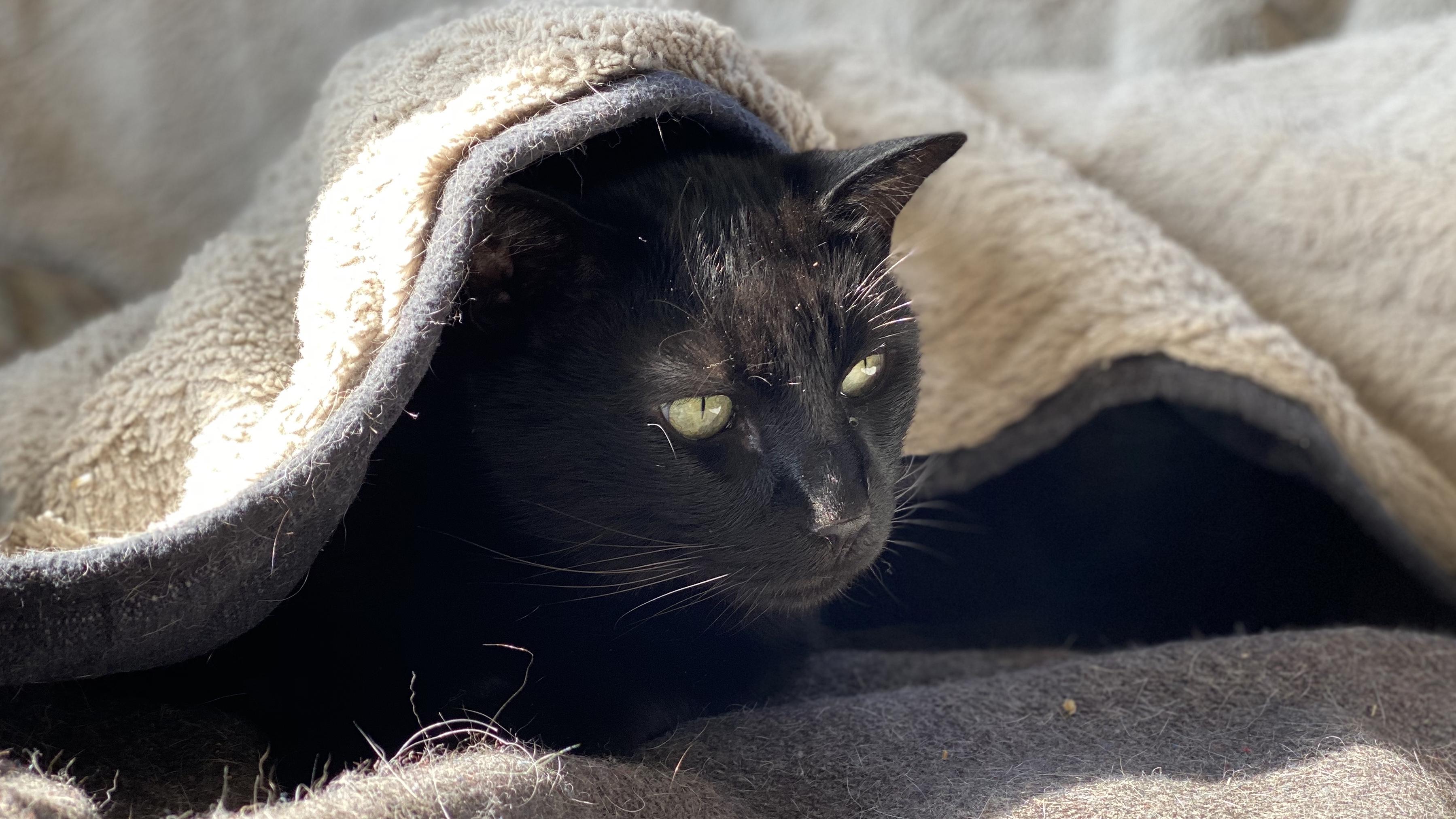
Caslon under the blanket

Caslon on the heater
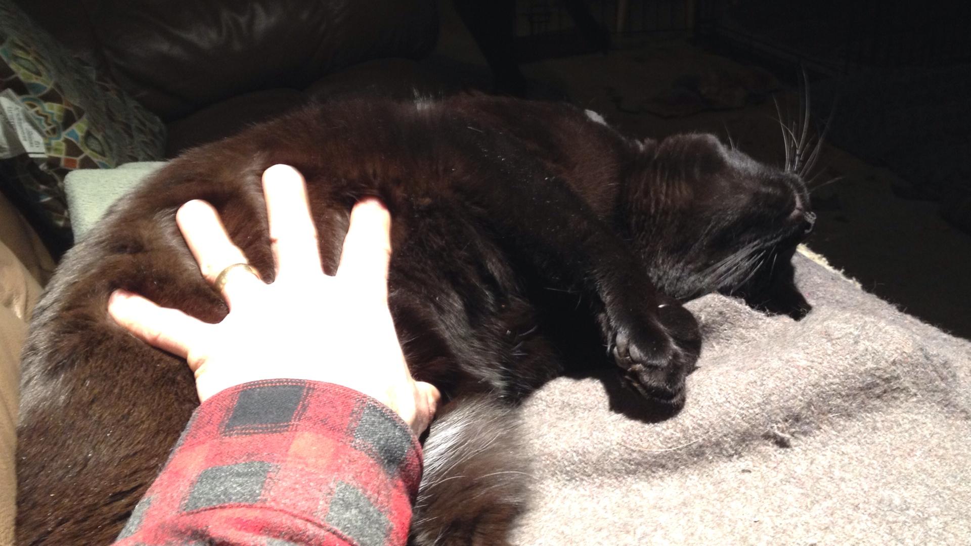
Belly pets
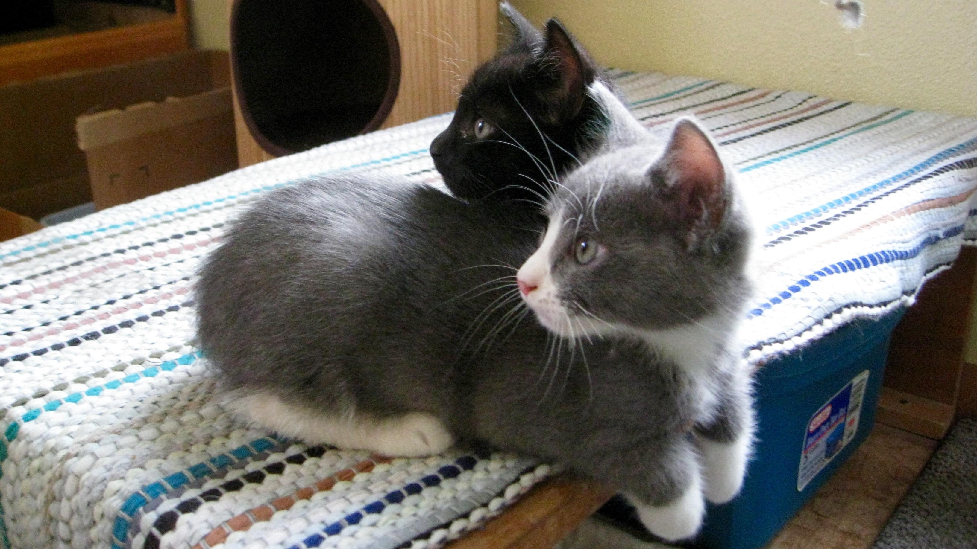
Caslon and Jenson
Introduction
Several years ago I wrote a post about Equinox Marathon weather, summarizing the conditions for all 50+ races. Since that post Andrea and I have run the relay twice, and I’ve run the full marathon three more times (if I include last year’s COVID-19 cancelled race). Despite no official race last year, quite a few people came out to run it in the rain and fog. This post updates the statistics and plots to include last year’s weather data.
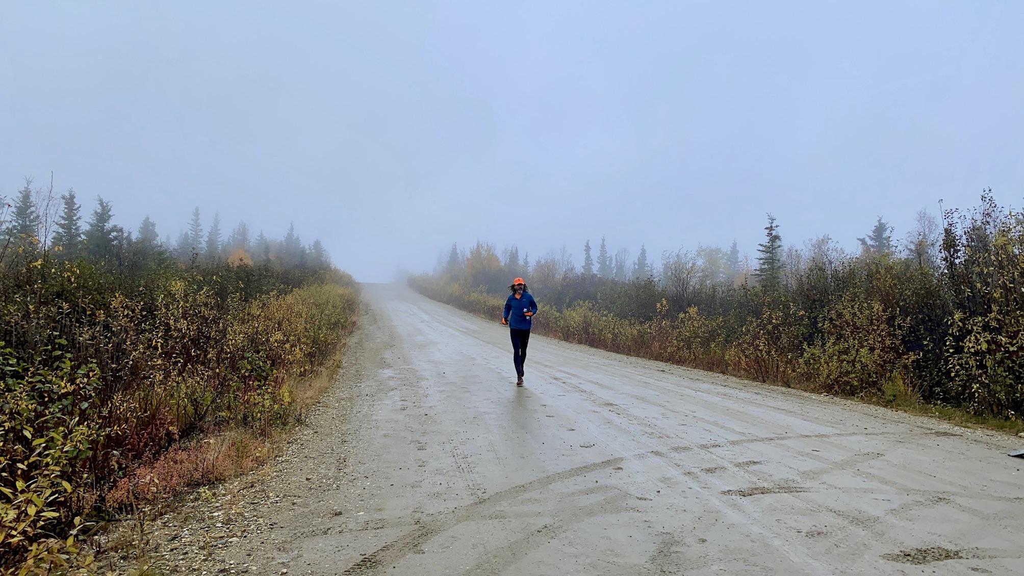
Conditions on Ester Dome during the 2020 marathon
Methods
Methods and data are the same as in my previous post, except the daily data has been updated to include years through 2020. The R code is available at the end of the previous post.
Results
Race day weather
Temperatures at the airport on race day ranged from 19.9 °F in 1972 to 68 °F in 1969, but the average range is between 34.5 and 53.0 °F. Using our model of Ester Dome temperatures, we get an average range of 29.8 and 47.3 °F and an overall min / max of 16.1 / 61.3 °F up on the Dome. Generally speaking, it will be below freezing on Ester Dome, but usually before most of the runners get up there.
Precipitation (rain, sleet or snow) has fallen on 18 out of 58 race days, or 31% of the time, and measurable snowfall has been recorded on four of those eighteen. The highest amount fell in 2014 with 0.36 inches of liquid precipitation (no snow was recorded and the temperatures were between 45 and 51 °F so it was almost certainly all rain, even on Ester Dome). More than a quarter of an inch of precipitation fell in three of the eighteen years when it rained or snowed (1990, 1993, and 2014), but most rainfall totals are much smaller.
Measurable snow fell at the airport in four years, or seven percent of the time: 4.1 inches in 1993, 2.1 inches in 1985, 1.2 inches in 1996, and 0.4 inches in 1992. But that’s at the airport station. Five of the 14 years where measurable precipitation fell at the airport and no snow fell, had possible minimum temperatures on Ester Dome that were below freezing. It’s likely that some of the precipitation recorded at the airport in those years was coming down as snow up on Ester Dome. If so, that means snow may have fallen on nine race days, bringing the percentage up to sixteen percent.
Wind data from the airport has only been recorded since 1984, but from those years the average wind speed at the airport on race day is 4.8 miles per hour. The highest 2-minute wind speed during Equinox race day was 21 miles per hour in 2003. Unfortunately, no wind data is available for Ester Dome, but it’s likely to be higher than what is recorded at the airport.
Weather from the week prior
It’s also useful to look at the weather from the week before the race, since excessive pre-race rain or snow can make conditions on race day very different, even if the race day weather is pleasant. The first year I ran the full marathon (2013), it snowed the week before and much of the trail in the woods before the water stop near Henderson and all of the out and back were covered in snow.
The most dramatic example of this was 1992 where 23 inches (!) of snow fell at the airport in the week prior to the race, with much higher totals up on the summit of Ester Dome. Measurable snow has been recorded at the airport in the week prior to six races, but all the weekly totals are under an inch except for the snow year of 1992.
Precipitation has fallen in 46 of 58 pre-race weeks (79% of the time). Three years have had more than an inch of precipitation prior to the race: 1.49 inches in 2015, 1.26 inches in 1992 (most of which fell as snow), and 1.05 inches in 2007. On average, just over two tenths of an inch of precipitation falls in the week before the race.
Summary
The following stacked plots shows the weather for all 58 runnings of the Equinox marathon. The top panel shows the range of temperatures on race day from the airport station (wide bars) and estimated on Ester Dome (thin lines below bars). The shaded area at the bottom shows where temperatures are below freezing. The orange horizonal lines represent average high and low temperature in the valley (dashed lines) and on Ester Dome (solid orange lines).
The middle panel shows race day liquid precipitation (rain, melted snow). Bars marked with an asterisk indicate years where snow was also recorded at the airport, but remember that five of the other years with liquid precipitation probably experienced snow on Ester Dome (1977, 1986, 1991, 1994, and 2016) because the temperatures were likely to be below freezing at elevation.
The bottom panel shows precipitation totals from the week prior to the race. Bars marked with an asterisk indicate weeks where snow was also recorded at the airport.

Here’s a table with most of the data from the analysis.
| Date | min t | max t | ED min t | ED max t | awnd | prcp | snow | p prcp | p snow |
|---|---|---|---|---|---|---|---|---|---|
| 1963-09-21 | 32.0 | 54.0 | 27.5 | 48.2 | 0.00 | 0.0 | 0.01 | 0.0 | |
| 1964-09-19 | 34.0 | 57.9 | 29.4 | 51.8 | 0.00 | 0.0 | 0.03 | 0.0 | |
| 1965-09-25 | 37.9 | 60.1 | 33.1 | 53.9 | 0.00 | 0.0 | 0.80 | 0.0 | |
| 1966-09-24 | 36.0 | 62.1 | 31.3 | 55.8 | 0.00 | 0.0 | 0.01 | 0.0 | |
| 1967-09-23 | 35.1 | 57.9 | 30.4 | 51.8 | 0.00 | 0.0 | 0.00 | 0.0 | |
| 1968-09-21 | 23.0 | 44.1 | 19.1 | 38.9 | 0.00 | 0.0 | 0.04 | 0.0 | |
| 1969-09-20 | 35.1 | 68.0 | 30.4 | 61.3 | 0.00 | 0.0 | 0.00 | 0.0 | |
| 1970-09-19 | 24.1 | 39.9 | 20.1 | 34.9 | 0.00 | 0.0 | 0.42 | 0.0 | |
| 1971-09-18 | 35.1 | 55.9 | 30.4 | 50.0 | 0.00 | 0.0 | 0.14 | 0.0 | |
| 1972-09-23 | 19.9 | 42.1 | 16.1 | 37.0 | 0.00 | 0.0 | 0.01 | 0.2 | |
| 1973-09-22 | 30.0 | 44.1 | 25.6 | 38.9 | 0.00 | 0.0 | 0.05 | 0.0 | |
| 1974-09-21 | 48.0 | 60.1 | 42.5 | 53.9 | 0.08 | 0.0 | 0.00 | 0.0 | |
| 1975-09-20 | 37.9 | 55.9 | 33.1 | 50.0 | 0.02 | 0.0 | 0.02 | 0.0 | |
| 1976-09-18 | 34.0 | 59.0 | 29.4 | 52.9 | 0.00 | 0.0 | 0.54 | 0.0 | |
| 1977-09-24 | 36.0 | 48.9 | 31.3 | 43.4 | 0.06 | 0.0 | 0.20 | 0.0 | |
| 1978-09-23 | 30.0 | 42.1 | 25.6 | 37.0 | 0.00 | 0.0 | 0.10 | 0.3 | |
| 1979-09-22 | 35.1 | 62.1 | 30.4 | 55.8 | 0.00 | 0.0 | 0.17 | 0.0 | |
| 1980-09-20 | 30.9 | 43.0 | 26.5 | 37.8 | 0.00 | 0.0 | 0.35 | 0.0 | |
| 1981-09-19 | 37.0 | 43.0 | 32.2 | 37.8 | 0.15 | 0.0 | 0.04 | 0.0 | |
| 1982-09-18 | 42.1 | 61.0 | 37.0 | 54.8 | 0.02 | 0.0 | 0.22 | 0.0 | |
| 1983-09-17 | 39.9 | 46.9 | 34.9 | 41.5 | 0.00 | 0.0 | 0.05 | 0.0 | |
| 1984-09-22 | 28.9 | 60.1 | 24.6 | 53.9 | 5.8 | 0.00 | 0.0 | 0.08 | 0.0 |
| 1985-09-21 | 30.9 | 42.1 | 26.5 | 37.0 | 6.5 | 0.14 | 2.1 | 0.57 | 0.0 |
| 1986-09-20 | 36.0 | 52.0 | 31.3 | 46.3 | 8.3 | 0.07 | 0.0 | 0.21 | 0.0 |
| 1987-09-19 | 37.9 | 61.0 | 33.1 | 54.8 | 6.3 | 0.00 | 0.0 | 0.00 | 0.0 |
| 1988-09-24 | 37.0 | 45.0 | 32.2 | 39.7 | 4.0 | 0.00 | 0.0 | 0.11 | 0.0 |
| 1989-09-23 | 36.0 | 61.0 | 31.3 | 54.8 | 8.5 | 0.00 | 0.0 | 0.07 | 0.5 |
| 1990-09-22 | 37.9 | 50.0 | 33.1 | 44.4 | 7.8 | 0.26 | 0.0 | 0.00 | 0.0 |
| 1991-09-21 | 36.0 | 57.0 | 31.3 | 51.0 | 4.5 | 0.04 | 0.0 | 0.03 | 0.0 |
| 1992-09-19 | 24.1 | 33.1 | 20.1 | 28.5 | 6.7 | 0.01 | 0.4 | 1.26 | 23.0 |
| 1993-09-18 | 28.0 | 37.0 | 23.8 | 32.2 | 4.9 | 0.29 | 4.1 | 0.37 | 0.3 |
| 1994-09-24 | 27.0 | 51.1 | 22.8 | 45.5 | 6.0 | 0.02 | 0.0 | 0.08 | 0.0 |
| 1995-09-23 | 43.0 | 66.9 | 37.8 | 60.3 | 4.0 | 0.00 | 0.0 | 0.00 | 0.0 |
| 1996-09-21 | 28.9 | 37.9 | 24.6 | 33.1 | 6.9 | 0.06 | 1.2 | 0.26 | 0.0 |
| 1997-09-20 | 27.0 | 55.0 | 22.8 | 49.1 | 3.8 | 0.00 | 0.0 | 0.03 | 0.0 |
| 1998-09-19 | 42.1 | 60.1 | 37.0 | 53.9 | 4.9 | 0.00 | 0.0 | 0.37 | 0.0 |
| 1999-09-18 | 39.0 | 64.9 | 34.1 | 58.4 | 3.8 | 0.00 | 0.0 | 0.26 | 0.0 |
| 2000-09-16 | 28.9 | 50.0 | 24.6 | 44.4 | 5.6 | 0.00 | 0.0 | 0.30 | 0.0 |
| 2001-09-22 | 33.1 | 57.0 | 28.5 | 51.0 | 1.6 | 0.00 | 0.0 | 0.00 | 0.0 |
| 2002-09-21 | 33.1 | 48.9 | 28.5 | 43.4 | 3.8 | 0.00 | 0.0 | 0.03 | 0.0 |
| 2003-09-20 | 26.1 | 46.0 | 22.0 | 40.7 | 9.6 | 0.00 | 0.0 | 0.00 | 0.0 |
| 2004-09-18 | 26.1 | 48.0 | 22.0 | 42.5 | 4.3 | 0.00 | 0.0 | 0.25 | 0.0 |
| 2005-09-17 | 37.0 | 63.0 | 32.2 | 56.6 | 0.9 | 0.00 | 0.0 | 0.09 | 0.0 |
| 2006-09-16 | 46.0 | 64.0 | 40.7 | 57.6 | 4.3 | 0.00 | 0.0 | 0.00 | 0.0 |
| 2007-09-22 | 25.0 | 45.0 | 20.9 | 39.7 | 4.7 | 0.00 | 0.0 | 1.05 | 0.0 |
| 2008-09-20 | 34.0 | 51.1 | 29.4 | 45.5 | 4.5 | 0.00 | 0.0 | 0.08 | 0.0 |
| 2009-09-19 | 39.0 | 50.0 | 34.1 | 44.4 | 5.8 | 0.00 | 0.0 | 0.25 | 0.0 |
| 2010-09-18 | 35.1 | 64.9 | 30.4 | 58.4 | 2.5 | 0.00 | 0.0 | 0.00 | 0.0 |
| 2011-09-17 | 39.9 | 57.9 | 34.9 | 51.8 | 1.3 | 0.00 | 0.0 | 0.44 | 0.0 |
| 2012-09-22 | 46.9 | 66.9 | 41.5 | 60.3 | 6.0 | 0.00 | 0.0 | 0.33 | 0.0 |
| 2013-09-21 | 24.3 | 44.1 | 20.3 | 38.9 | 5.1 | 0.00 | 0.0 | 0.13 | 0.6 |
| 2014-09-20 | 45.0 | 51.1 | 39.7 | 45.5 | 1.6 | 0.36 | 0.0 | 0.00 | 0.0 |
| 2015-09-19 | 37.9 | 44.1 | 33.1 | 38.9 | 2.9 | 0.01 | 0.0 | 1.49 | 0.0 |
| 2016-09-17 | 34.0 | 57.9 | 29.4 | 51.8 | 2.2 | 0.01 | 0.0 | 0.61 | 0.0 |
| 2017-09-16 | 33.1 | 66.0 | 28.5 | 59.5 | 3.1 | 0.00 | 0.0 | 0.02 | 0.0 |
| 2018-09-15 | 44.1 | 60.1 | 38.9 | 53.9 | 3.8 | 0.00 | 0.0 | 0.00 | 0.0 |
| 2019-09-21 | 37.0 | 45.0 | 32.2 | 39.7 | 7.6 | 0.13 | 0.0 | 0.40 | 0.0 |
| 2020-09-19 | 39.9 | 53.1 | 34.9 | 47.3 | 2.2 | 0.12 | 0.0 | 0.10 | 0.0 |